Sanctions

library(tidyverse)

── Attaching core tidyverse packages ──────────────────────── tidyverse 2.0.0 ──
✔ dplyr     1.2.1     ✔ readr     2.2.0
✔ forcats   1.0.1     ✔ stringr   1.6.0
✔ ggplot2   4.0.3     ✔ tibble    3.3.1
✔ lubridate 1.9.5     ✔ tidyr     1.3.2
✔ purrr     1.2.2     
── Conflicts ────────────────────────────────────────── tidyverse_conflicts() ──
✖ dplyr::filter() masks stats::filter()
✖ dplyr::lag()    masks stats::lag()
ℹ Use the conflicted package (<http://conflicted.r-lib.org/>) to force all conflicts to become errors

library(readxl)
library(ggplot2)

#install.packages("tidyverse")
gsdb = readr::read_csv(here::here("data", "raw", "GSDB_V4.csv"))

Rows: 1547 Columns: 16
── Column specification ────────────────────────────────────────────────────────
Delimiter: ","
chr  (5): sanctioned_state, sanctioning_state, descr_trade, objective, success
dbl (11): case_id, begin, end, trade, arms, military, financial, travel, oth...

ℹ Use `spec()` to retrieve the full column specification for this data.
ℹ Specify the column types or set `show_col_types = FALSE` to quiet this message.

ties = readxl::read_excel(here::here("data", "raw", "TIESv4-1.xls"))

max_year <- max(gsdb$end, na.rm = TRUE)

gsdb_expanded <- gsdb %>%
  # Create a sequence of years from 'begin' to 'end' for each row
  mutate(year = map2(begin, end, ~seq(.x, .y))) %>%
  # Expand the list of years into individual rows
  unnest(cols = c(year))

# Aggregate the active sanctions per year
gsdb_type_counts <- gsdb_expanded %>%
  group_by(year) %>%
  summarise(across(
    c(trade, arms, military, financial, travel, other), 
    ~sum(.x, na.rm = TRUE)
  )) %>%
  # Pivot from wide to long format for ggplot2
  pivot_longer(
    cols = -year, 
    names_to = "sanction_type", 
    values_to = "count"
  ) %>% 
  mutate(sanction_type = fct_reorder(sanction_type, count, .fun = sum, .desc = TRUE))

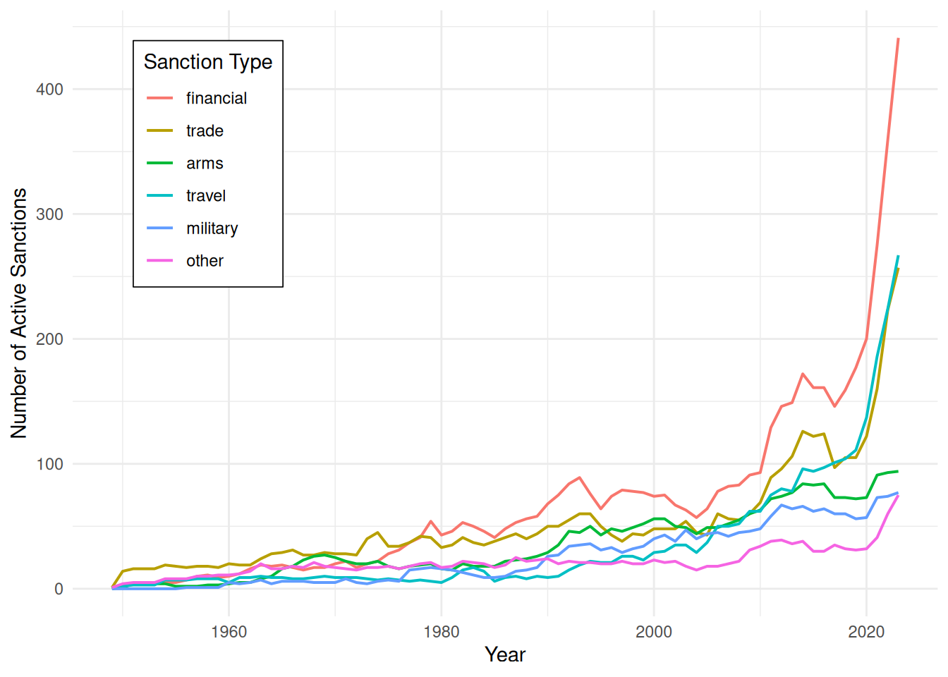
# Plot the data
ggplot(gsdb_type_counts, aes(x = year, y = count, color = sanction_type)) +
  geom_line(linewidth = .7) +
  labs(
    x = "Year",
    y = "Number of Active Sanctions",
    color = "Sanction Type"
  ) +
  theme_minimal() +
  theme(
    legend.position = c(0.07, 0.95), 
    legend.justification = c("left", "top"), 
    legend.background = element_rect(fill = "white", color = "black", linewidth = 0.3), 
    axis.title = element_text(size = 11)
  )

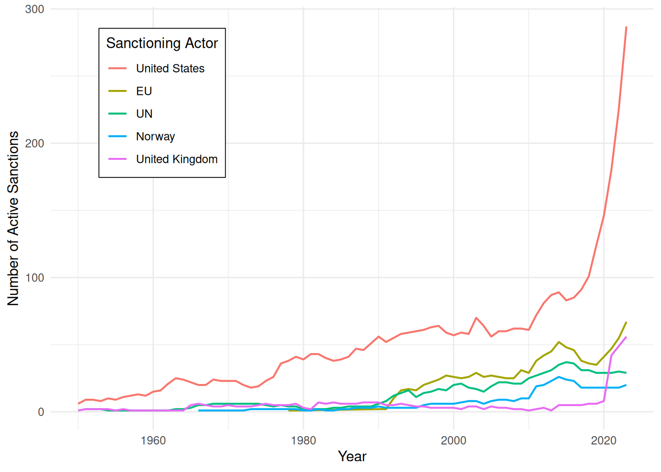
# Separate the actors and aggregate
gsdb_actor_counts <- gsdb_expanded %>%
  separate_longer_delim(sanctioning_state, delim = ", ") %>%
  group_by(year, sanctioning_state) %>%
  summarise(count = n(), .groups = "drop")

# Filter for top 10 actors with the most sanction-years 
top_actors <- gsdb_actor_counts %>%
  group_by(sanctioning_state) %>%
  summarise(total = sum(count)) %>%
  slice_max(total, n = 5) %>%
  pull(sanctioning_state)

gsdb_actor_counts_filtered <- gsdb_actor_counts %>%
  filter(sanctioning_state %in% top_actors) %>% 
  mutate(sanctioning_state = fct_reorder(sanctioning_state, count, .fun = sum, .desc = TRUE))

# Plot the data
ggplot(gsdb_actor_counts_filtered, aes(x = year, y = count, color = sanctioning_state)) +
  geom_line(linewidth = .7) +
  labs(
    x = "Year",
    y = "Number of Active Sanctions",
    color = "Sanctioning Actor"
  ) +
  theme_minimal() +
  theme(
    legend.position = c(0.08, 0.95), 
    legend.justification = c("left", "top"), 
    legend.background = element_rect(fill = "white", color = "black", linewidth = 0.3), 
    axis.title = element_text(size = 11)
  )