HowWarsEnd

library(dplyr)

Attaching package: 'dplyr'

The following objects are masked from 'package:stats':

    filter, lag

The following objects are masked from 'package:base':

    intersect, setdiff, setequal, union

#install.packages("tidyverse")
termination_data = readr::read_csv(here::here("data", "raw", "UCDPConflictTerminationDataset_v4_2024_Conflict.csv"))

Rows: 2752 Columns: 36
── Column specification ────────────────────────────────────────────────────────
Delimiter: ","
chr  (13): location, side_a, side_a_id, side_a_2nd, side_b, side_b_id, side_...
dbl  (20): conflict_id, incompatibility, year, intensity_level, cumulative_i...
date  (3): start_date, start_date2, c_ependdate

ℹ Use `spec()` to retrieve the full column specification for this data.
ℹ Specify the column types or set `show_col_types = FALSE` to quiet this message.

conflict_data = readr::read_csv(here::here("data", "raw", "UcdpPrioConflict_v25_1.csv"))

Rows: 2752 Columns: 28
── Column specification ────────────────────────────────────────────────────────
Delimiter: ","
chr  (14): location, side_a, side_a_id, side_a_2nd, side_b, side_b_id, side_...
dbl  (10): conflict_id, incompatibility, year, intensity_level, cumulative_i...
lgl   (1): ep_end_prec
date  (3): start_date, start_date2, ep_end_date

ℹ Use `spec()` to retrieve the full column specification for this data.
ℹ Specify the column types or set `show_col_types = FALSE` to quiet this message.

Variables of interest:

type of conflict2 The same conflict episode, or dyadic conflict episode, may include both years where neither side receive secondary support and years when they do. Type 2 thus combine the categories of internal armed conflict and internationalized armed conflict into the categories described below 1. Extrasystemic armed conflict. 2. Interstate armed conflict. 3. Intrastate armed conflict.

c outcome The coding of outcomes are based on the final year of activity and first year of non-activity. 1= Peace agreement 2= Ceasefire 3= Victory for Side A /Government Side 4= Victory for Side B /Non-State Side 5= Low activity (some, but less than 25 battle-deaths in subsequent year(s)) 6= Actor ceases to exist

termination_data <- termination_data %>%
  mutate(c_outcome_simple = case_when(
    is.na(c_outcome)           ~ "ongoing",
    c_outcome %in% c(1, 2)     ~ "diplomatic",
    c_outcome %in% 3:6         ~ "military",
    TRUE                       ~ "other"  # Catch-all for unexpected values
  ))

# create decade variable and termination variable
termination_data <- termination_data %>%
  mutate(decade = (year %/% 10) * 10) 


termination_data <- termination_data %>%
  # Sort by ID and Year to ensure 'lead' picks the correct next row
  arrange(conflict_id, year) %>%
  
  # Group by ID so we only compare years within the same conflict
  group_by(conflict_id) %>%
  
  # Create the duration (gap) variable
  mutate(duration = ifelse(
    c_epterm == 1, 
    lead(year) - year, 
    NA
  )) %>%
  ungroup()

termination_data <- termination_data %>%
  # Ensure data is ordered correctly by conflict and time
  arrange(conflict_id, year) %>%
  group_by(conflict_id) %>%
  mutate(
    # 1. Create conflict_resumes
    # Check if any subsequent year exists for this conflict_id
    conflict_resumes = ifelse(
      c_epterm == 1, 
      as.integer(year < max(year)), 
      NA
    ),
    # 2. Create peace_duration
    # Calculate years until the next recorded observation for this conflict
    peace_duration = ifelse(
      c_epterm == 1 & conflict_resumes == 1,
      lead(year) - year,
      NA
    )
  ) %>%
  ungroup()

termination_data <- termination_data %>%   
  mutate(
    # 1. Create conflict_resumes
    # Check if any subsequent year exists for this conflict_id
    peace_never_fails = ifelse(
      c_epterm == 1 & is.na(peace_duration), 
      as.integer(max(year)-year), 
      NA
    )
  )

termination_data <- termination_data %>%   
  mutate(
    # 1. Create conflict_resumes
    # Check if any subsequent year exists for this conflict_id
    peace_fails_in_10 = ifelse(
      c_epterm == 1 & (peace_duration>10 | is.na(peace_duration)), 
      0, 
      1
    )
  )

library(ggplot2)

ggplot(termination_data %>% filter(type_of_conflict %in% c(2, 4)), 
       aes(x = year, fill = c_outcome_simple)) +
  geom_bar(position = "stack") +
  scale_x_continuous(
    breaks = seq(from = 1900, to = 2020, by = 10) # Adjust start/end to your data
  ) +
  labs(
    title = "War Terminations Each Year by Outcome",
    x = "Year",
    y = "Wars Terminated",
    fill = "Outcome Type"
  ) +
  theme_minimal()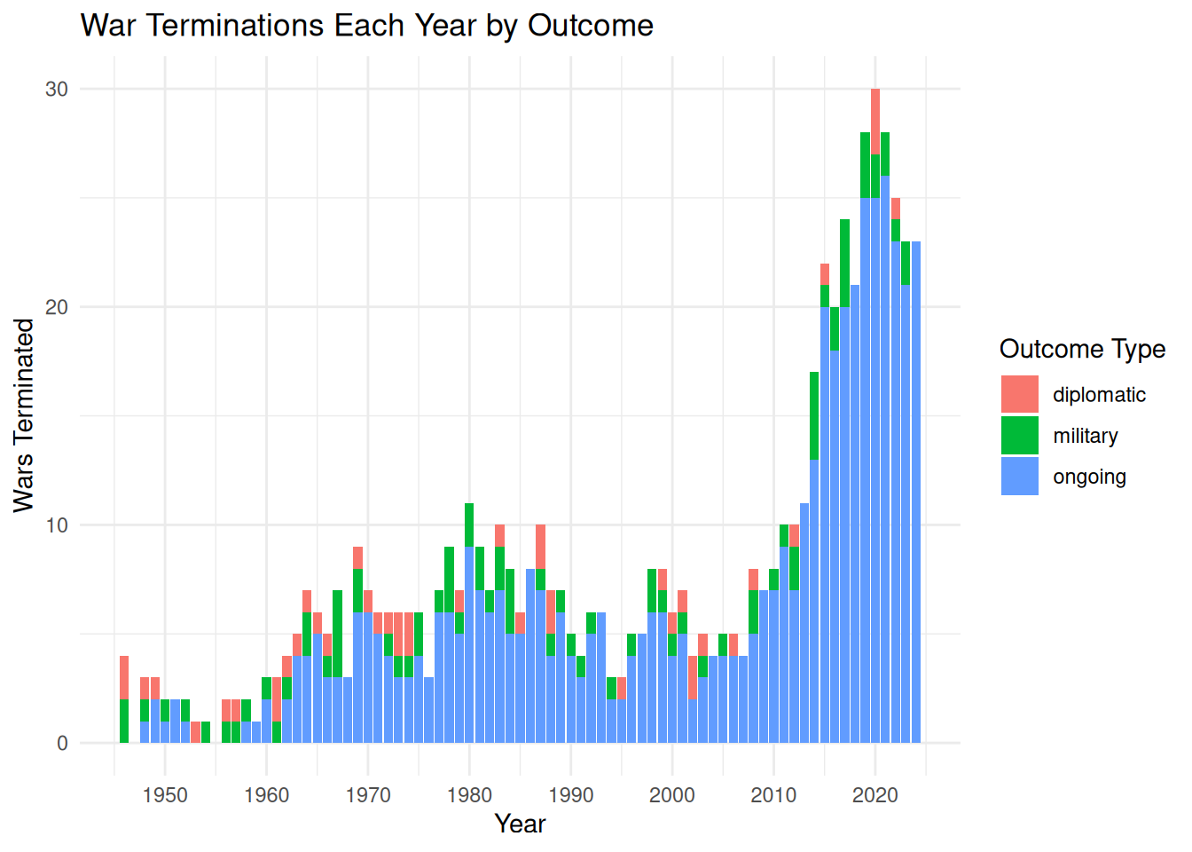

# Pre-calculate the counts per year and outcome

decade_data <- termination_data %>% 
  filter(c_outcome_simple != 'ongoing') %>%
  filter(type_of_conflict == 2 | type_of_conflict == 4) %>%
  mutate(decade = (year %/% 10) * 10) 

# Create the line chart
ggplot(decade_data, aes(x = decade, fill = c_outcome_simple)) +
  geom_bar(position = "stack") +
  scale_x_continuous(breaks = seq(from = 1900, to = 2020, by = 10)) +
  labs(
    title = "War Terminations Over Time by Outcome",
    x = "Year",
    y = "Number of Wars Terminated",
    color = "Outcome Type"
  ) +
  theme_minimal()

Ignoring unknown labels:
• colour : "Outcome Type"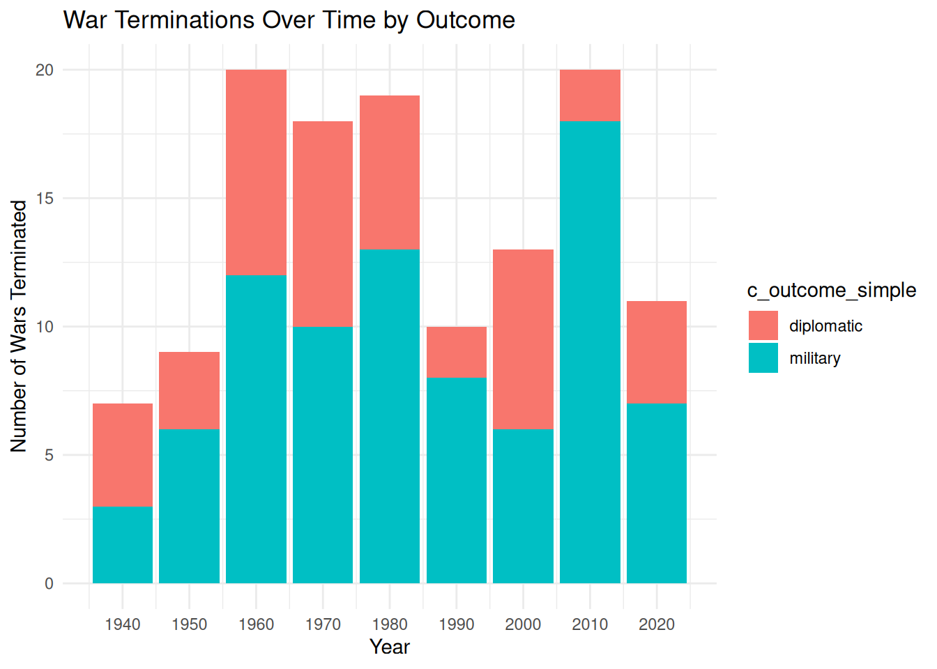

Outcomes of Interstate Wars

# Pre-calculate the counts per year and outcome
decade_data <- termination_data %>% 
  filter(c_outcome_simple != 'ongoing') %>%
  filter(type_of_conflict == 2 ) %>%
  mutate(decade = (year %/% 10) * 10)

# Get counts
decade_data

# A tibble: 72 × 43
   conflict_id location  side_a side_a_id side_a_2nd side_b side_b_id side_b_2nd
         <dbl> <chr>     <chr>  <chr>     <chr>      <chr>  <chr>     <chr>     
 1         214 France, … Gover… 33        <NA>       Gover… 147       <NA>      
 2         215 Albania,… Gover… 45        <NA>       Gover… 28        <NA>      
 3         218 India, P… Gover… 141       <NA>       Gover… 142       <NA>      
 4         218 India, P… Gover… 141       <NA>       Gover… 142       <NA>      
 5         218 India, P… Gover… 141       <NA>       Gover… 142       <NA>      
 6         218 India, P… Gover… 141       <NA>       Gover… 142       <NA>      
 7         218 India, P… Gover… 141       <NA>       Gover… 142       <NA>      
 8         218 India, P… Gover… 141       <NA>       Gover… 142       <NA>      
 9         218 India, P… Gover… 141       <NA>       Gover… 142       <NA>      
10         218 India, P… Gover… 141       <NA>       Gover… 142       <NA>      
# ℹ 62 more rows
# ℹ 35 more variables: incompatibility <dbl>, territory_name <chr>, year <dbl>,
#   intensity_level <dbl>, cumulative_intensity <dbl>, type_of_conflict <dbl>,
#   start_date <date>, start_prec <dbl>, start_date2 <date>, start_prec2 <dbl>,
#   gwno_a <chr>, gwno_a_2nd <chr>, gwno_b <dbl>, gwno_b_2nd <chr>,
#   gwno_loc <chr>, region <chr>, type_of_conflict2 <dbl>, c_epid <dbl>,
#   c_epno <dbl>, c_ep_startyear <dbl>, c_epterm <dbl>, c_outcome <dbl>, …

# Create the line chart
ggplot(decade_data, aes(x = decade, fill = c_outcome_simple)) +
  geom_bar(position = "stack") +
  scale_x_continuous(breaks = seq(from = 1900, to = 2020, by = 10)) +
  labs(
    # title = "War Terminations Over Time by Outcome",
    x = "Decade",
    y = "Number of Wars Terminated",
    color = "Outcome Type",
    fill = "Means of War End"
  ) +
  theme_minimal() +
  theme(
    # Move legend inside the plot area (top right)
    legend.position = c(0.98, 0.98),
    # Anchor the legend by its top-right corner so it doesn't bleed off the edge
    legend.justification = c("right", "top"),
    # Optional: Add a background/border to ensure readability against the bars
    legend.background = element_rect(fill = "white", color = "black", linewidth = 0.2),
    axis.title = element_text(size = 11, color = "black"),
    axis.text = element_text(size = 11, color = "black")
  )

Ignoring unknown labels:
• colour : "Outcome Type"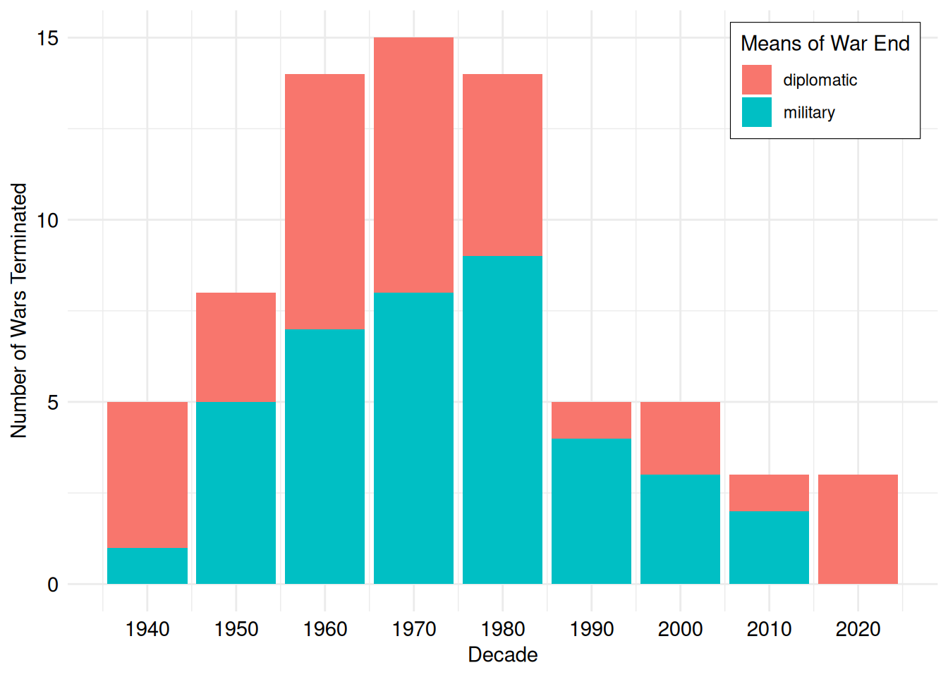

# total number of conflicts
termination_data %>% filter(type_of_conflict == 2) %>% select(conflict_id) %>% unique() %>% nrow()

[1] 52

decade_count <- termination_data %>% 
  filter(c_outcome_simple != 'ongoing') %>%
  filter(type_of_conflict == 2) %>%
  count(decade, c_outcome_simple)

# count of interstate conflict endins for whole dataset

decade_count %>%
  group_by(c_outcome_simple) %>%         
  summarize(total_n = sum(n))

# A tibble: 2 × 2
  c_outcome_simple total_n
  <chr>              <int>
1 diplomatic            33
2 military              39

termination_data %>% 
  filter(c_outcome_simple != 'ongoing') %>%
  filter(type_of_conflict == 2) %>%
  group_by(c_outcome_simple, conflict_resumes) %>%
  summarize(total_n = n(), .groups = 'drop')

# A tibble: 4 × 3
  c_outcome_simple conflict_resumes total_n
  <chr>                       <int>   <int>
1 diplomatic                      0      24
2 diplomatic                      1       9
3 military                        0      24
4 military                        1      15

termination_data %>% 
  filter(c_epterm == 1) %>%
  filter(c_outcome_simple != 'ongoing') %>%
  filter(type_of_conflict == 2) %>%
  filter(conflict_resumes == 1) %>%
  group_by(c_outcome_simple) %>%         
  summarize(
    count = n(),
    avg_peace = mean(peace_duration, na.rm = TRUE),
    .groups = "drop" # Keeps the output as a clean, ungrouped tibble
  )

# A tibble: 2 × 3
  c_outcome_simple count avg_peace
  <chr>            <int>     <dbl>
1 diplomatic           9      10  
2 military            15       8.4

termination_data %>% 
  filter(c_epterm == 1) %>%
  filter(c_outcome_simple != 'ongoing') %>%
  filter(type_of_conflict == 2) %>%
  filter(conflict_resumes == 1) %>% 
  select(c_outcome_simple, peace_duration) %>% 
  arrange(peace_duration)

# A tibble: 24 × 2
   c_outcome_simple peace_duration
   <chr>                     <dbl>
 1 military                      2
 2 military                      2
 3 military                      2
 4 military                      2
 5 military                      2
 6 military                      2
 7 military                      2
 8 military                      3
 9 diplomatic                    3
10 military                      4
# ℹ 14 more rows

termination_data %>% 
  filter(c_epterm == 1) %>%
  filter(c_outcome_simple != 'ongoing') %>%
  filter(type_of_conflict == 2) %>%
  filter(conflict_resumes == 1) %>%
  group_by(c_outcome_simple, peace_fails_in_10) %>%         
  summarize(
    count = n(),
    avg_peace = mean(peace_duration, na.rm = TRUE),
    .groups = "drop" # Keeps the output as a clean, ungrouped tibble
  )

# A tibble: 4 × 4
  c_outcome_simple peace_fails_in_10 count avg_peace
  <chr>                        <dbl> <int>     <dbl>
1 diplomatic                       0     4     14.5 
2 diplomatic                       1     5      6.4 
3 military                         0     2     43   
4 military                         1    13      3.08

termination_data %>% 
  filter(c_epterm == 1) %>%
  filter(c_outcome_simple != 'ongoing') %>%
  filter(type_of_conflict == 2) %>%
  group_by(c_outcome_simple, peace_fails_in_10) %>%         
  summarize(
    count = n(),
    avg_peace = mean(peace_duration, na.rm = TRUE),
    .groups = "drop" # Keeps the output as a clean, ungrouped tibble
  )

# A tibble: 4 × 4
  c_outcome_simple peace_fails_in_10 count avg_peace
  <chr>                        <dbl> <int>     <dbl>
1 diplomatic                       0    28     14.5 
2 diplomatic                       1     5      6.4 
3 military                         0    26     43   
4 military                         1    13      3.08

termination_data %>% 
  filter(c_epterm == 1) %>%
  filter(c_outcome_simple != 'ongoing') %>%
  filter(type_of_conflict == 2) %>%
  group_by(c_outcome_simple) %>%         
  summarize(
    count = n(),
    percent_fail = mean(peace_fails_in_10),
    .groups = "drop" # Keeps the output as a clean, ungrouped tibble
  )

# A tibble: 2 × 3
  c_outcome_simple count percent_fail
  <chr>            <int>        <dbl>
1 diplomatic          33        0.152
2 military            39        0.333

Outcomes of Interstate and Internationalized Wars

# Create the line chart
ggplot(termination_data %>%
    filter(c_outcome_simple != 'ongoing') %>%
    filter(type_of_conflict %in% c(2,4)), 
  aes(x = decade, fill = c_outcome_simple)) +
  geom_bar(position = "stack") +
  scale_x_continuous(breaks = seq(from = 1900, to = 2020, by = 10)) +
  labs(
    title = "War Terminations Over Time by Outcome",
    x = "Year",
    y = "Number of Wars Terminated",
    color = "Outcome Type"
  ) +
  theme_minimal()

Ignoring unknown labels:
• colour : "Outcome Type"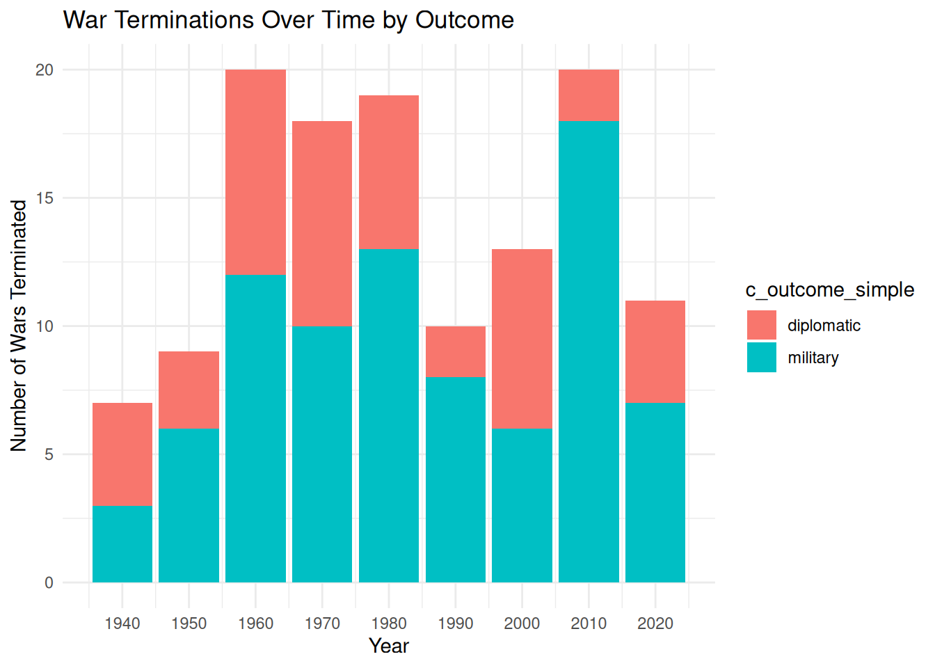

decade_plus_count <- termination_data %>% 
  filter(c_outcome_simple != 'ongoing') %>%
  filter(type_of_conflict %in% c(2,4)) %>%
  count(decade, c_outcome_simple)

decade_plus_count %>%
  filter(decade > 1999) %>%     
  group_by(c_outcome_simple) %>%         
  summarize(total_n = sum(n))

# A tibble: 2 × 2
  c_outcome_simple total_n
  <chr>              <int>
1 diplomatic            13
2 military              31

decade_plus_count %>%
  group_by(c_outcome_simple) %>%         
  summarize(total_n = sum(n))

# A tibble: 2 × 2
  c_outcome_simple total_n
  <chr>              <int>
1 diplomatic            44
2 military              83

Duration of peace

restart_analysis <- termination_data %>%
  filter(type_of_conflict %in% c(2,4)) %>%
  filter(c_outcome_simple %in% c("diplomatic", "military")) %>%
  filter(c_epterm == 1) %>%
  
  # Group by the type of termination
  group_by(c_outcome_simple) %>%
  
  # Calculate the metrics
  summarize(
    total_terminations = n(),
    num_restarts = sum(!is.na(duration)),
    avg_peace_duration = mean(duration, na.rm = TRUE)
  )

print(restart_analysis)

# A tibble: 2 × 4
  c_outcome_simple total_terminations num_restarts avg_peace_duration
  <chr>                         <int>        <int>              <dbl>
1 diplomatic                       44           15               8.73
2 military                         83           37               6.43

restart_analysis <- termination_data %>%
  filter(type_of_conflict %in% c(2,4)) %>%
  filter(decade > 1999) %>%     
  filter(c_outcome_simple %in% c("diplomatic", "military")) %>%
  filter(c_epterm == 1) %>%
  
  # Group by the type of termination
  group_by(c_outcome_simple) %>%
  
  # Calculate the metrics
  summarize(
    total_terminations = n(),
    num_restarts = sum(!is.na(duration)),
    avg_peace_duration = mean(duration, na.rm = TRUE)
  )

print(restart_analysis)

# A tibble: 2 × 4
  c_outcome_simple total_terminations num_restarts avg_peace_duration
  <chr>                         <int>        <int>              <dbl>
1 diplomatic                       13            5               9.4 
2 military                         31           15               3.47

Scrap

ggplot(termination_data %>% 
         filter(c_outcome_simple != 'ongoing') %>% 
           filter(type_of_conflict == 4), 
       aes(x = year, fill = c_outcome_simple)) +
  geom_bar(position = "stack") +
  scale_x_continuous(
    breaks = seq(from = 1900, to = 2020, by = 10) # Adjust start/end to your data
  ) +
  labs(
    title = "War Terminations Each Year by Outcome",
    x = "Year",
    y = "Wars Terminated",
    fill = "Outcome Type"
  ) +
  theme_minimal()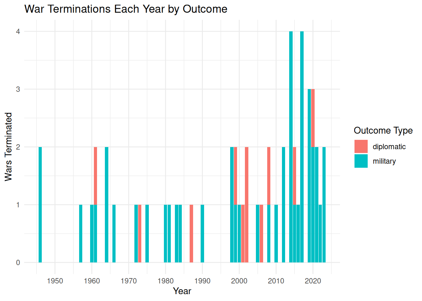

ggplot(termination_data %>% 
         filter(c_outcome_simple != 'ongoing') %>% 
           filter(type_of_conflict == 2), 
       aes(x = year, fill = c_outcome_simple)) +
  geom_bar(position = "stack") +
  scale_x_continuous(
    breaks = seq(from = 1900, to = 2020, by = 10) # Adjust start/end to your data
  ) +
  labs(
    title = "War Terminations Each Year by Outcome",
    x = "Year",
    y = "Wars Terminated",
    fill = "Outcome Type"
  ) +
  theme_minimal()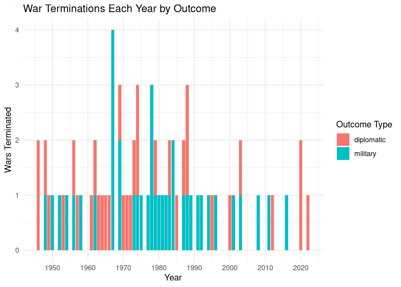

# Pre-calculate the counts per year and outcome

plot_data <- termination_data %>% 
  filter(c_outcome_simple != 'ongoing') %>%
  count(year, c_outcome_simple)

# Create the line chart 
ggplot(plot_data, aes(x = year, y = n, color = c_outcome_simple)) +
  geom_line(linewidth = 1) +
  scale_x_continuous(
    breaks = seq(from = 1900, to = 2020, by = 10)
  ) +
  labs(
    title = "War Terminations Over Time by Outcome",
    x = "Year",
    y = "Number of Wars Terminated",
    color = "Outcome Type"
  ) +
  theme_minimal()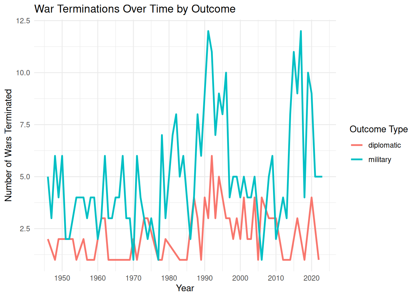

# Pre-calculate the counts per year and outcome
plot_data <- termination_data %>% 
  filter(c_outcome_simple != 'ongoing') %>%
  filter(type_of_conflict == 2) %>%
  count(year, c_outcome_simple)

# Create the line chart

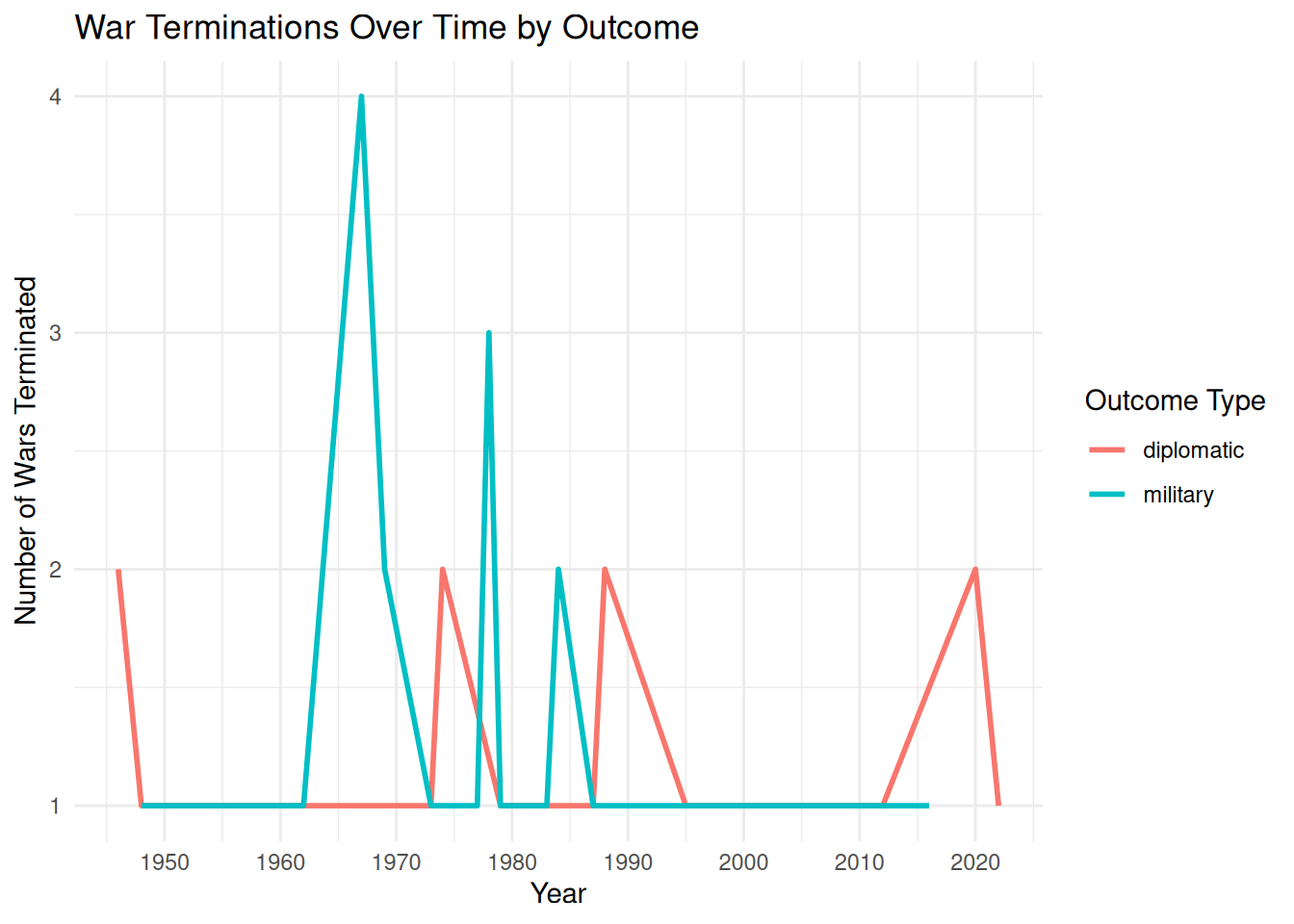
ggplot(plot_data, aes(x = year, y = n, color = c_outcome_simple)) +
  geom_line(linewidth = 1) +
  scale_x_continuous(
    breaks = seq(from = 1900, to = 2020, by = 10)
  ) +
  labs(
    title = "War Terminations Over Time by Outcome",
    x = "Year",
    y = "Number of Wars Terminated",
    color = "Outcome Type"
  ) +
  theme_minimal()